AnyWave:H2

Purpose

The plugin computes the connectivity between channels using h2/r2 algorithms.
It will produce a .mat file containing the results. This file can be then processed either in MATMAB or with the Correlation Graphs plugin of AnyWave.

How to run

Channels of interest

Before running the plugin, make sure you have selected the channels of interest.
If no channels are selected before running the plugin, you will get a warning message. Computing on many channels can lead to a long calculation as many pairs of channels must be considered.

Data selection

Mark the data of interest with one or more markers.
It's a good practice to give the markers an explicit name.

Run

There are two ways to run the plugin:

• Running using the Processes menu of AnyWave.
• Running user the markers GUI.

If you have marked data, you can specify which artefacted parts of the data to avoid in computation using the skip data using markers options:

• select the marker corresponding to the part to skip (ie 'artefact').
• click Skip button to add it to the list of markers to skip.

In the same way, you can also specify on which particular marked data compute the connectivity:

• select the marker corresponding to a period of interest.
• click the Use button to add it to the list of markers to use for computation.

Frequency bands

You can compute the connectivity on different frequency bands.
By default, the AnyWave band is selected which means the filter options set in AnyWave will be used.
You can enable the different predefined bands and even change the frequency boundaries.

Review resulting graphs

When the computation is finished, the resuslts are saved to a MATLAB file located in the data file's folder.
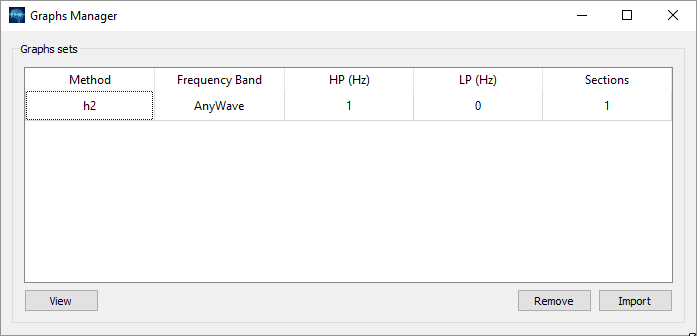
Another plugin is automatically launched allowing you to browse the different connectivy graphs:

The UI propose all the graphs resulting from the computation. A graph for each frequency band.
You can see what algorihtm was used on what frequency band and the number of sections which is the number of selected part of data used for computation.

Click on rows to select them and click on View to see the graphs.

Batch mode

The plugin is able to run in batch mode.
See this section for more details

json settings for h2/r2:

{ 
"plugin" : "h2",
"algorithm" : "r2",
"time_window" : 4,
"max_lag" : 0.1,
"step" : 1,
"downsampling_factor" : 2,
"output_prefix" : "my_result"
}

Common options that can also be specified in the command line if you want to apply them to a specific file and not ALL the files:

key	description	default behavior
marker_file	path to the .mrk file to use	if not specified, AnyWave will try to locate the .mrk associated with the data file and use it.
use_markers	array of marker labels to use	optional but may required marker_file option.
skip_markers	array of marker labels to SKIP (artefacts)	optional but may required marker_file option.
hp	high pass filter in Hz	optional
lp	low pass filter in Hz	optional

H2 specific options:

key	description	requirement	default behavior
plugin	Name of plugin	MANDATORY	n/a
time_window	the time window in s.	MANDATORY	n/a
max_lag	maximum lag in s.	MANDATORY	n/a
step	step in s.	MANDATORY	n/a
downsampling_factor	downsampling data	OPTIONAL	default is 1. 2 means the sampling rate of the data will be divided by 2.
output_prefix	prefix of resulting file name	OPTIONAL	default is no prefix.

Example

using this json file:

{ 
"plugin" : "h2",
"algorithm" : "r2",
"time_window" : 4,
"max_lag" : 0.1,
"step" : 1,
"downsampling_factor" : 2,
"output_prefix" : "my_result",
"use_markers" : [ "EI" ]
}

We will compute on a file stored in D:\Data\

anywave --run h2.json --input_file d:\data\data_file.eeg --marker_file d:\data\data_file.mrk --hp 1 --lp 45

This will compute compute r2 values for the file data_file.eeg using 1-45Hz frequency band only on data marked by a EI marker.