Difference between revisions of "AnyWave:H2"
(→variables) |
(→The result file) |
||
| Line 155: | Line 155: | ||
* year, month, day : recorded date (may contain weird values if the data file does not contain a valid recording date.) | * year, month, day : recorded date (may contain weird values if the data file does not contain a valid recording date.) | ||
* hour, minute, second : recorded time (may contain weird values if the data file does not contain a valid recording time.) | * hour, minute, second : recorded time (may contain weird values if the data file does not contain a valid recording time.) | ||
| − | + | ==Notice== | |
| − | + | ||
No matters the number of markers set as input, all the results are stacked in the matrices.<br/> | No matters the number of markers set as input, all the results are stacked in the matrices.<br/> | ||
So for two markers which don't overlap each other, there will be two sections in the .mat file.<br/> | So for two markers which don't overlap each other, there will be two sections in the .mat file.<br/> | ||
Latest revision as of 15:36, 9 August 2019
Contents
Purpose
The plugin computes the connectivity between channels using h2/r2 algorithms.
It will produce a .mat file containing the results. This file can be then processed either in MATLAB or by the Correlation Graphs plugin of AnyWave.
Data input
channels
This plugin requires at least two channels as input.
The user can select the channels of interest in the signal view before running the plugin.
NOTE: if no selection exists when running the plugin then ALL the channels will be set as input: A warning prompt will ask you to confirm that.
markers
The user may also used markers to select the different part of data on which to compute.
It is possible to run the plugin on selected markers or to use the Main GUI once the plugin has started to specify the data input.
NOTE: if there is no suitable marker (either no markers at all or markers with no duration) then the plugin will compute on the whole data.
How to run
Step 1 - Selected channels of interest:
Before running the plugin, make sure you have selected the channels of interest.
If no channels are selected before running the plugin, you will get a warning message.
Computing on many channels can lead to long calculation as many pairs of channels must be considered.
Step 2 - Select data of interest:
Mark the data of interest with one or more markers.
It's a good practice to give the markers an explicit name.
Step 3 - Run the plugin:
There are two ways to run the plugin:
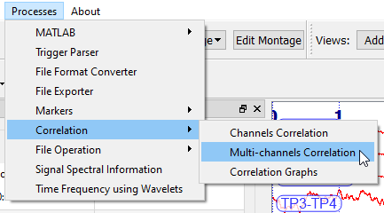
- Running using the Processes menu of AnyWave.
- Running from the markers GUI.
Run from markers
Select the markers of interest in the widget, then right click and pick the plugin to run.

Main GUI

Computation parameters:
Change here the computation method (h² or r²) and the timing parameters.
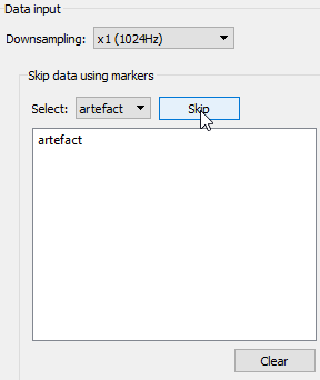
Data input:
- Step 1 (OPTIONAL) : reduce computation time by downsampling the data.
By default the ratio is 1 meaning that no downsampling will be applied.
Change the ratio if you want to reduce computation time.
- Step 2 : skip AND/OR use markers (this section will be hidden if you have launched the the plugin using the markers).
Avoiding artefacted data (OPTIONAL):
Pick a marker name that matches an artefacted region in the data and click the skip button to add it to the main list of markers to avoid.
All the markers with that name will be skipped.

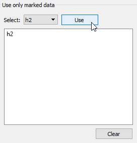
Using markers:
Pick a marker name that matches data region you want to use and click the Use button to add the name to the main list of markers to use.

In our example we will compute the correlations on all markers named h2 avoiding markers named artefact that may overlapped the h2 markers.
IMPORTANT: If you dont specify markers to use, the plugin will use ALL the markers available (with a duration).
Frequency bands
You can compute the connectivity on different frequency bands.
By default, the AnyWave band is selected which means the filter options set in AnyWave will be used.
You can enable the different predefined bands and even change the frequency boundaries.
Run in batch mode
The plugin is able to run in batch mode.
You will need to write a shell script and create a json file.
See this section for more details
json settings for h2/r2:
{
"plugin" : "h2",
"algorithm" : "r2",
"time_window" : 4,
"max_lag" : 0.1,
"step" : 1,
"downsampling_factor" : 2,
"output_prefix" : "my_result"
}
Common options that can also be specified in the command line if you want to apply them to a specific file and not ALL the files:
| key | description | default behavior |
|---|---|---|
| marker_file | path to the .mrk file to use | if not specified, AnyWave will try to locate the .mrk associated with the data file and use it. |
| use_markers | array of marker labels to use | optional but may require marker_file option. |
| skip_markers | array of marker labels to SKIP (artefacts) | optional but may require marker_file option. |
| hp | high pass filter in Hz | optional |
| lp | low pass filter in Hz | optional |
H2 specific options:
| key | description | requirement | default behavior |
|---|---|---|---|
| plugin | Name of plugin | MANDATORY | n/a |
| time_window | the time window in s. | MANDATORY | n/a |
| max_lag | maximum lag in s. | MANDATORY | n/a |
| step | step in s. | MANDATORY | n/a |
| downsampling_factor | downsampling data | OPTIONAL | default is 1. 2 means the sampling rate of the data will be divided by 2. |
| output_prefix | prefix of resulting file name | OPTIONAL | default is no prefix. |
Example
using this json file:
{
"plugin" : "h2",
"algorithm" : "r2",
"time_window" : 4,
"max_lag" : 0.1,
"step" : 1,
"downsampling_factor" : 2,
"output_prefix" : "my_result",
"use_markers" : [ "EI" ]
}
We will compute on a file stored in D:\Data\
anywave --run h2.json --input_file d:\data\data_file.eeg --marker_file d:\data\data_file.mrk --hp 1 --lp 45
This will compute compute r2 values for the file data_file.eeg using 1-45Hz frequency band only on data marked by EI markers.
The result file
The plugin will generate a MATLAB file named using the data file name as a prefix.
The name will also contain the frequency band defined and the algorithm used to compute.
NOTE: If several frequency bands where defined in the main GUI, the plugin will generate a result file for each of the frequency band.
variables
The MATLAB file contains the following variables:
- aw_h2 : a 3D matrix containing the correlation values. The dimensions are n x n x it (where n is the number of channels and it the number of time windows computed)
- aw_lag : a 3D matrix containing the lag values. Same dimensions than aw_h2.
- aw_maxLag : reminder of the max lag parameter used.
- aw_step : reminder of the step parameter used.
- aw_windowSize : reminder of the time_window paremeter used.
- band : a string containing the name of the frequency band used. This variable is empty if the plugin ran in batch mode.
- electrode_names : ordered labels of all channels.
- filters : values of the frequency band used.
- nb_section : The total number of data parts used by the plugin.
- section : an index vector containing the section number of each slices in the 3D matrices. (WARNING indexes start at zero).
- section_iterations : a vector containing the total number of iterations (or slices) for each sections.
- time : a vector containing the sample index of each slices in the 3D matrices.
- time_s : a vector containing the position in seconds in the file of each slices of the 3D matrices.
- samplingRate : sampling rate of the data.
- method : the algorithm used.
- year, month, day : recorded date (may contain weird values if the data file does not contain a valid recording date.)
- hour, minute, second : recorded time (may contain weird values if the data file does not contain a valid recording time.)
Notice
No matters the number of markers set as input, all the results are stacked in the matrices.
So for two markers which don't overlap each other, there will be two sections in the .mat file.
However, all the time windows computed are stacked in the matrix. Each slice is an iteration of a sections.
Using the section vector will give you the section number (starting at zero) of a slice in the matrices.
That way, it is possible to get the correlation values through time.
